Some Notes on Nonparametric Statistics of the Komogorov-Smirnov Class

All physical processes have variability. In the past hundred years scientists and mathematicians have devised many methods for “seeing through” variability to the underlying principles. “Statistics” is the art devised to help deal with variability.

It is usual in introductory statistics to focus on models for variability and it is usual for students to learn about “average”, and “standard deviation” and bell curves. It is less usual for students to have real laboratory data to deal with. Real data rapidly teaches that bell curves are few and far between. People who have never spent time in a laboratory taking data can be forgiven for believing that most distributions are Gaussian since this is usually all they know.

The use of “average” and “standard deviation” presumes certain kinds of distributions, usually Gaussian, also known as the Normal distribution. (The word “Normal” here does not mean “usual”, it means “independent”.) So while it can be useful to know what the distribution of a sample is, it is often not necessary. Much of the time all you want to know is whether two samples are different, and/or if one sample (the outputs of some process) is larger or smaller than some other sample.

To deal with variability in the real world one must start with non-parametric statistics, that is, statistics that do not presume any particular distribution. It is never appropriate to assume that a new distribution is Gaussian without testing.

A powerful and simple nonparametric method for comparing distributions or for comparing distributions to functions is the class of Kolmogorov-Smirnov (K-S) statistics. K-S tests are a sort of statistical multi-tool. The Lillefors test for normality uses the K-S method to compare a sample to the cumulative curve represented by the average and standard deviation of the data

The basic idea is easy. Construct the empirical and/or theoretical cumulative distributions, and then look at the maximum difference between the distributions projected onto the cumulative axis. This difference is the statistic for the test. All K-S statistics are based on this maximum distance between cumulative curves along the cumulative axis.

The use of cumulatives avoids the need to “bucket” or group the data. This puts the representation of continuous and disconcontinuous functions on a parallel basis. For the X axis, or non cumulative axis, you can transform the data to suit your purposes. It does not change the statistical test.

Even for cases where parametric statistics are appropriate, the K-S statistic still works, though sometimes with less “statistical power” than a focussed parametric test. But there are few tests with the general power and utility of the K-S type statistics. If you learn nothing else about statistics, I urge learning how to use the various K-S tests.

In statistics, a “sample” means a set of numbers, and for the K-S tests the numbers must be continuously distributed, that is, real numbers. Duplicates should be unlikely. Duplicates may invalidate the K-S tests.

There may be some issues with regard to nomenclature. My 1970 book by W. J.Conover, “Practical Nonparametric Statistics” calls the two random sample test the Smirnov Test, and the comparison between one random sample and a function with no degrees of freedom the Kolmogorov Test. Calling the two sample test a K-S test creates no logical problem except for figuring out what significance table or function to use.

First let’s look at a comparison of a function with a sample using the Microsoft Excel random number generator. We expect that the cumulative distribution for the uniform number generator to be a straight line between zero and one.

ExcelRandom

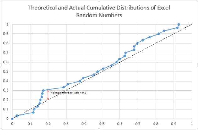
For this test, the (one sample) Kolmogorov statistic is 0.1. As a crude approximation 1/sqrt(N)= 0.18 is the 80% significance level, so as far as this test goes, we can presume the generator to be “uniform”, that is, the sample is not significantly different from the expected continuous distribution.

Let’s look at an example of a classic problem: Fisher’s analysis of Darwin’s data on “fertilisation”

Darwin2

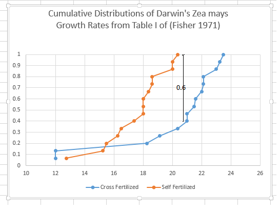
I cite the example not to disparage the great geneticist Sir Ronald Fisher, who was brilliant for his day, but to show how much progress has been made in dealing with variability. In his classic book, “The Design of Experiments”** , Fisher discusses some data of Darwin on the breeding of plants. Darwin was trying to show that cross fertilisation (I assume we would say pollination) was better than self fertilisation. Fisher shows some data, and says (pp 38) “that for these data, t > 2.148, or significant at the 5% level, that is barely significant”. Darwin wanted the difference to be significant, the more the better. Given the great variability, Darwin had been uncertain of the outcome. Subjecting the same data to the Smirnov two sample one sided test, it is clear that the distributions differ by 9/15. Thus it is less than 0.5% probability that the two data sets are from the same distribution. The cross fertilized were quite significantly bigger. This conclusion was far less clear in the early 20th century.

Summary of K-S Related Tests

( A “sample” means a group of numbers originating from some process.)

(The term “one sided” means we want to know only if either the function or sample is significantly greater or lesser, but not both.)

(A “parameter” is a number used to define a distribution. Average, standard deviation, skewness, kurtosis are all parameters.)

To test a function with no parameters estimated from the data against a sample, use the Kolmogorov Test, also called the Kolmogorov-Smirnov one sample test. The function can have its own parameters, but these must be independent of the data being tested.

To test two samples against each other use the Smirnov Test, also called the Kolmogorov-Smirnov two sample test.

To test a function with one parameter estimated from the sample, use the Lillefors exponential function test.

To test a function with two parameters estimated from the data such as average and standard deviation use the Lillefors test for normality


Global Energy Flux Distributions

It is certainly true that most of the heat delivered by the sun leaves the earth as radiation.

And so most discussions of global warming focus on the radiative properties of the planet.

But the usual planetary averages leave out a lot of details. One of these details is the substantial movement of heat energy within the atmosphere. The screen capture  shows 4 Mollweide projections.

The top two are of the solar insolation averaged over January and June 2015. The bottom two are similar projections for the outgoing long wave radiation. The top four projections have the same color scale, 0 to 400 W/M^2

First look at the top two, and see the dramatic difference in insolation between June and January.  But the bottom two for the outgoing radiation are quite similar. Clearly lots of energy has to move within the atmosphere to spread out all the heat.

A large part of the energy moves as water vapor and is released when the water condenses. The third row of Mollweide projections below shows the average rainfall for the previous months, expressed as watts per square meter using the formula 1mm H2O = 29 w/m^2.  Note that the Jan. and June plots are almost identical — the radiative forcing has been averaged out.  The scale below is a bit different from the top, 0-500W/M^2

RAINFALL

All data comes from https://neo.sci.gsfc.nasa.gov. Note that the site has caveats on the utility of .csv format.


Global Warming in Perspective

I thank Coyote for noting the need to compare temperature anomalies to real temperatures.

We start with a view of global warming to date.  Current estimates for future warming vary, but are on the order of  0.11 degree C per decade.

HadCRUT4

The HadCrut4 chart shows warming beginning in 1900. Clearly CO2 cannot be the only source of warming.

Now lets look at some real data of the sort you might read on your thermometer.

Data is from Weather Underground, https://www.wunderground.com/history/

Chicago2014

The little circle contains a scaled version of the HadCrut4 chart with the same vertical scale (4 pixels per degree F).

Given that the range of variation on a daily basis is tens of degrees, and on an annual basis a 100 degrees, even multiples of the historical warming would be hard to observe in real data.


Atmospheric Energy and Global Temperature

In discussions of climate, the use of a statistic “temperature anomaly” has become ubiquitous.  Further, the statistic has taken on the role of temperature in the minds of many people and in many NOAA press releases and web sites. But “temperature anomaly” is not a  temperature in any technical sense of the word “temperature”.  A discussion is presented by Essex, McKitrick, and Andresen (EMA) below.

“Temperature” is only defined rigorously for a system at equilibrium, so the action of adding different temperatures by definition denies the validity of all but, at most, one.

If an effect of CO2 is to somehow change the water content of air or to change wind speeds,  averaging temperatures will not show the correct change  in atmospheric heat content.

The measure of heat energy for a fluid is enthalpy.  In joules per kilogram,  the expression for total specific energy,  enthalpy + potential + kinetic is

h = (Cp * T – .026) + q * (L(T) + 1.84 * T) + g * Z + V2/2

Cp is heat capacity, T is temperature in Celsius, q is specific humidity in kg H20/kg dry air, g is gravity, L(T) is latent heat of water ~2501 kJ/kg , Z is altitude, V is wind speed.  All variables should be concurrent. Using average values does not produce an accurate “average enthalpy”, though a properly constructed average q might.

Enthalpy can be converted to an equivalent temperature with or without the potential and kinetic energy terms.  Adding the wind energy seems to make a “wet stagnation” temperature.

T equivalent = h /Cp

An interesting study is https://pielkeclimatesci.files.wordpress.com/2009/10/r-290.pdf
Pielke shows that the real world difference between equivalent temperature h/Cp and thermometer temperature can be tens of degrees Celsius.

Classical climate data often does not include the humidity data consistent with the temperature data needed to calculate atmospheric energy to an accuracy better than several percent. This inaccuracy is greater than effects attributable to CO2. Hurricane velocity winds add single degrees of effective temperature, but modest winds can add tenths of degrees.  Evaporation or condensation of water can change temperature by tens of degrees.

For a more formal discussion of wet enthalpy,

Click to access Thermodynamics%20Notes.pdf

Equivalent Temperature

Since enthalpy is an extensive property,  enthalpies of different systems can be added. To construct a regional or global equivalent temperature from a variety of enthalpies, we need two sums: the enthalpies times their mass weight factor, and the weight factors.

T equivalent =  (∑ hi ρ / ∑ ρ )/ Cp

where  ρ  is the mass density and hi is the enthalpy at a point i in the atmosphere.

While we do not have mass densities, we do have the numbers to calculate it:

ρ =  P / (RM T)   where Rm is  R/ effective molecular weight.

Effective molecular weight is   Q Mair + (1-Q) Mwater  where Mair and Mwater are molecular  weights, Q is the ratio of water density to air density, and P is pressure at the point of measure of temperature T.   Note that meteorological pressures are often corrected to sea level and need to be corrected back to the relevant altitude.

T  equivalent =  ∑ hi P / (RM T)   / ( ∑ P / (RM T) ) / Cp

P and Rm will all vary from point to point as well as h.

Largely because of the latent heat of water, the equivalent temperature can be much higher than thermometer temperature.  The following graph is for a variety of cities and times of day using data from  https://www.wunderground.com/history/, and uses the excellent formulas of Massen.  The upper  branch includes humid Key West FL. The lower branch includes the relatively dry Denver, CO.

EquivalentTemperature

Errors in Global Temperature Anomalies

The word “error” implies some standard from which the observed statistic differs.
It is common in statistics to use error as a measure of the extent to which a particular statistic varies from its expected value. In engineering, error means deviation from specification or design.  So the extent of error depends on the intended use.

For purposes of estimating ground radiation,  unmolested temperature is best but averaging of multiple sites should be weighted as T^4.    For estimating global heat content enthalpy+wind energy+potential energy should be used.,

If the purpose of calculating global temperature anomalies is to observe some heating effect from alteration of radiative transport by CO2,  and some heat is diverted to evaporation of water, then the observed temperatures do not accurately represent the heat effect.   Using Massen’s equations (below) for enthalpy adjusted for relative humidity(Rh)  and differentiating wrt  measured temperature and humidity, we find that the delta in measured temperature from an delta in relative humidity evaluated at 50%Rh and 15 oC(59 oF) is:

delta observed Temp/ delta %Rh  = (dh/d%Rh)/(dh/dTemp)  = 0.83 degc/%Rh

This means that, if the actual Rh is 1% higher than some reference standard, the observed temperature will be lower than its energy equivalent by 0.83oC since heat is locked up in creating water vapor.

Since dTemp/d%Rh varies with both humidity and temperature, an estimate of the degree to which humidity changes at constant enthalpy  requires consideration of all relevant variables.  All relations are highly non-linear and there is no expectation that errors will “average out”.

I speculate that part of the reason for the never ending adjustment of historical temperatures is an attempt to compensate for the inaccuracies inherent in temperature only estimates of energy.

References

Guest Post “Calculating Moist Enthalpy From Usual Meteorological Measurements By Francis Massen

Massen:  http://meteo.lcd.lu/papers/Enthalpy/calculating_moist_enthalpy_revisited.pdf

EMA: http://www.uoguelph.ca/~rmckitri/research/globaltemp/GlobTemp.JNET.pdf

Parts of this post were presented at   https://wattsupwiththat.com/2017/02/22/through-the-looking-glass-with-nasa-giss/#comment-2435373 and https://wattsupwiththat.com/2017/04/23/the-meaning-and-utility-of-averages-as-it-applies-to-climate/#comment-2484011